

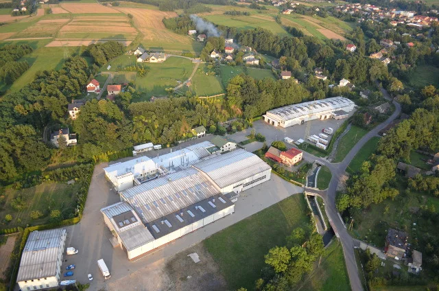
Improving OEE does not always begin with replacing a machine, increasing speed or adding a buffer. Czanieckie Makarony’s case study shows the value of first understanding variability across the line and testing a proposed investment in a digital twin. Only then can the organisation assess which solution will actually increase process capacity.
This article is based on Patryk Dybał’s presentation at Lean TWI Summit 2026 in Wrocław (2026 event, in Polish). The company presented a practical example of using MES data and a simulation model to evaluate development options for a production line. The key lesson goes beyond technology: a digital twin’s value lies in making a better decision before changing the real process.
Improving OEE at Czanieckie Makarony: the starting point
Czanieckie Makarony is a family business founded in 1990 by Władysław and Zbigniew Dybał. According to the conference materials, it employs approximately 250 people, produces approximately 10,000 tonnes of pasta annually and now involves the family’s third generation in managing the business. More about its quality standards and manufacturing process is available on the official Czanieckie Makarony website (in Polish).
The company faced a question familiar to growing FMCG plants: how to increase an existing line’s capacity when average productivity is not the only constraint. The process was fast but unstable. It varied over time because of people’s behaviour, breaks, minor faults and deliberate throttling of selected workstations. A static calculation could indicate average capacity, but could not show how variability travelled through the entire flow.
The question was not “Does a buffer work?” but “In which process configuration will a buffer actually increase line capacity?”
Improving OEE requires looking beyond averages
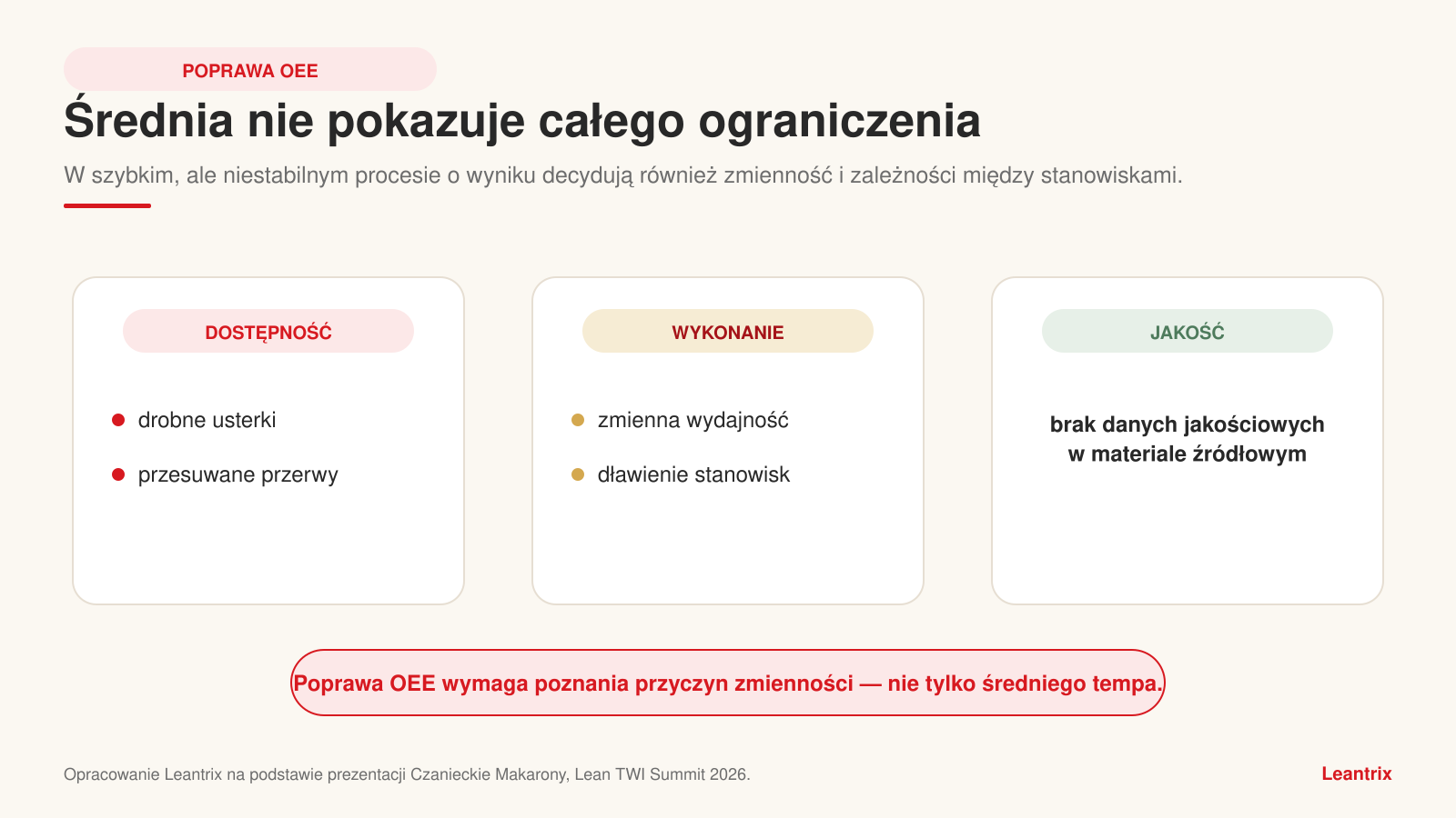
OEE combines three dimensions: availability, performance and quality. In practice, a single final percentage can conceal very different mechanisms. A minor breakdown reduces availability. Deliberate slowing or variable speed affects performance. Defects and rework reduce quality. When a team sees only the final result, it can easily select a solution for a symptom rather than a cause.
Czanieckie Makarony’s presentation did not publish quality data or an OEE increase in percentage points. This article therefore does not attribute an unsupported result to the company. It shows how variability analysis, model validation and scenario comparison can support decisions aimed at improving OEE, particularly availability and performance.
Four sources of process instability
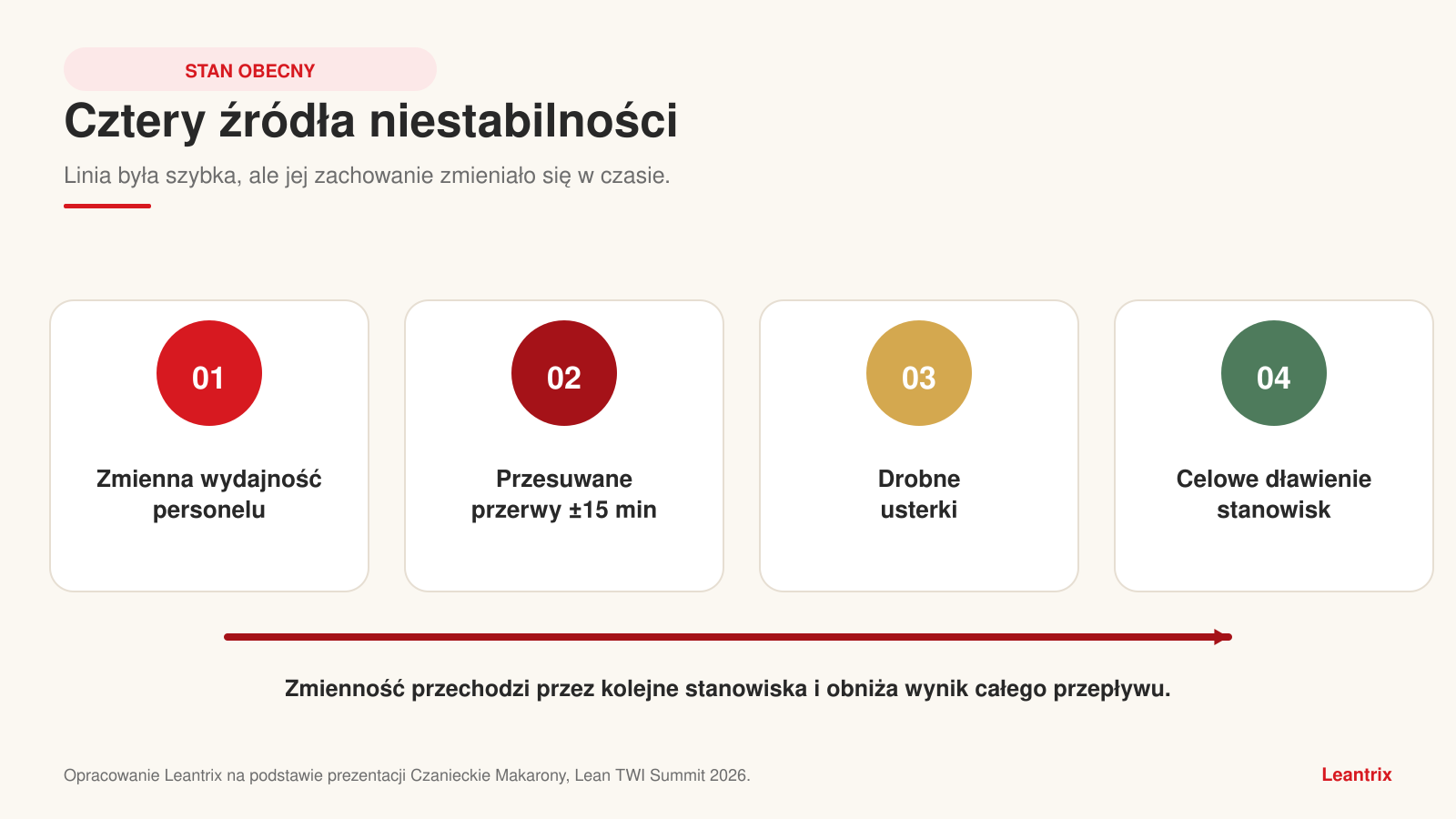
The presentation described four phenomena that made a simple investment appraisal difficult. Each may appear minor, but their combination changes the behaviour of the whole line.
- Workforce productivity varying over time. Average pace does not capture variations during a shift or their impact on downstream workstations.
- Breaks shifted by approximately 15 minutes. Changing break timing affects resource availability and the distribution of workload through the flow.
- Minor faults. Individual short events may seem unimportant, but their frequency and coincidence with other losses matter.
- Deliberate workstation throttling. Controlling the pace of one section protects the process locally but may restrict total line output.
As a result, two shifts with similar averages can follow completely different patterns. One may be stable; the other may contain frequent short accumulations and waiting periods. An investment decision based only on averages cannot see event sequences or how losses reinforce one another.
From an investment idea to a target-state question
The original challenge was increasing line capacity. A buffer was one option under consideration. Static calculations could not reliably predict its value in variable conditions. The company therefore faced the risk of spending money on a solution that looked reasonable on paper but might not deliver the expected result.
The target state was not defined as “buy a buffer”. The objective was a reliable basis for a decision. The digital twin was intended to answer two questions: whether the investment would increase line capacity, and what its scope should be to work with the other elements of the process.
Improving OEE: three steps in working with a digital twin
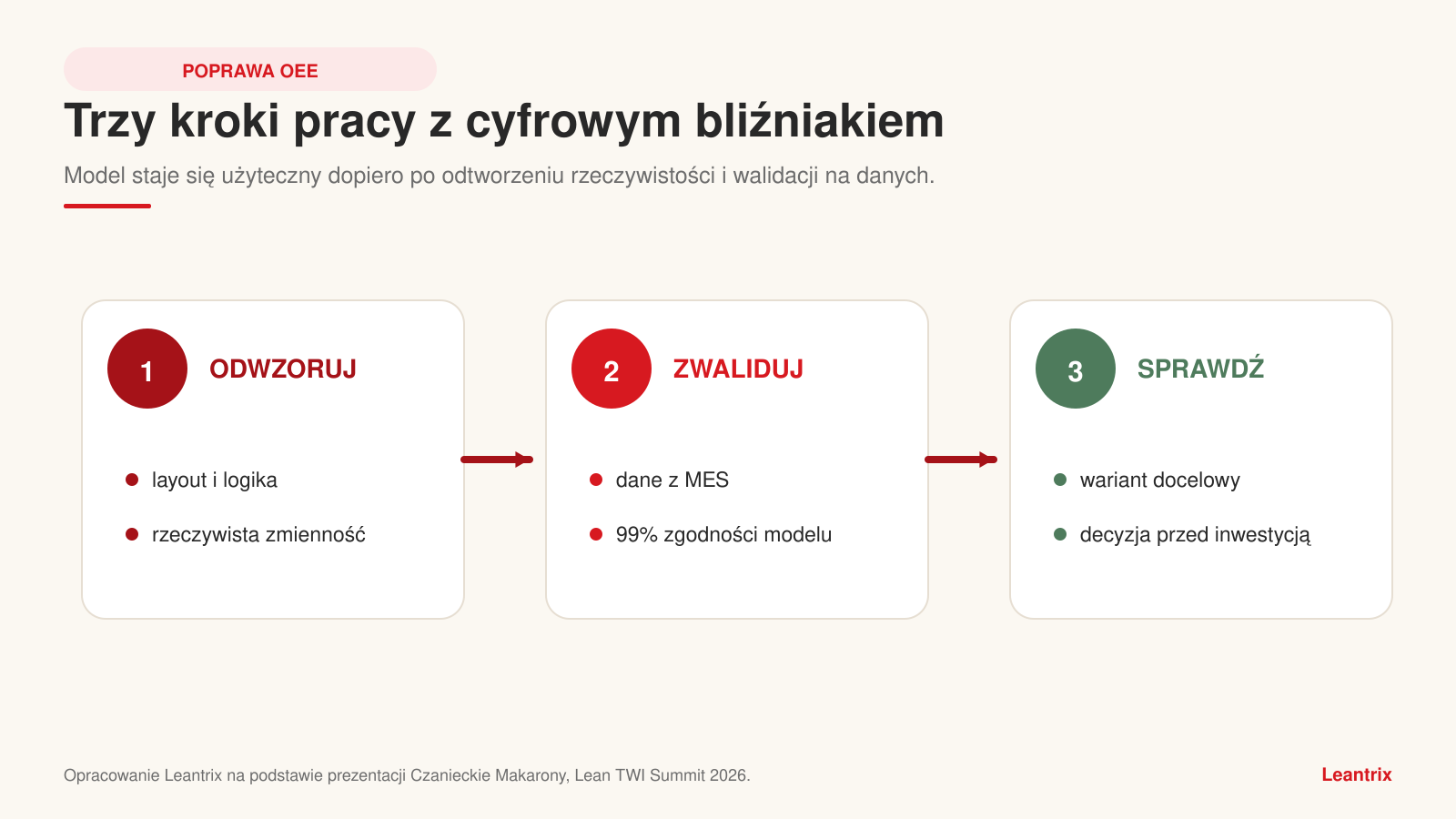
The team structured its approach into three steps. The sequence was essential: before testing the future, the model had to reproduce the actual process and be validated against data.
1. Representing the current state
The first digital-twin version was based on the line layout. Automation logic was then added, including throttling and direction changes. The model incorporated actual productivity variability over time and variable workstation staffing. It was therefore an attempt to reproduce real behaviour, rather than an elegant animation of an ideal process.
2. Validating the model with MES data
The model went through several iterations using actual MES data. The presentation reported 99% agreement between the model and reality. This validation level allowed the simulation to serve as a credible environment for comparing options rather than an approximate visualisation.
3. Representing the target state
Only after validation did the team model a working buffer and its intended logic. Data from earlier runs was used to ask a counterfactual question: what would the same shifts’ results have looked like if the buffer had already existed? Scenarios could then be compared without stopping production or incurring the full investment cost.
Improving OEE: five layers of a credible production model
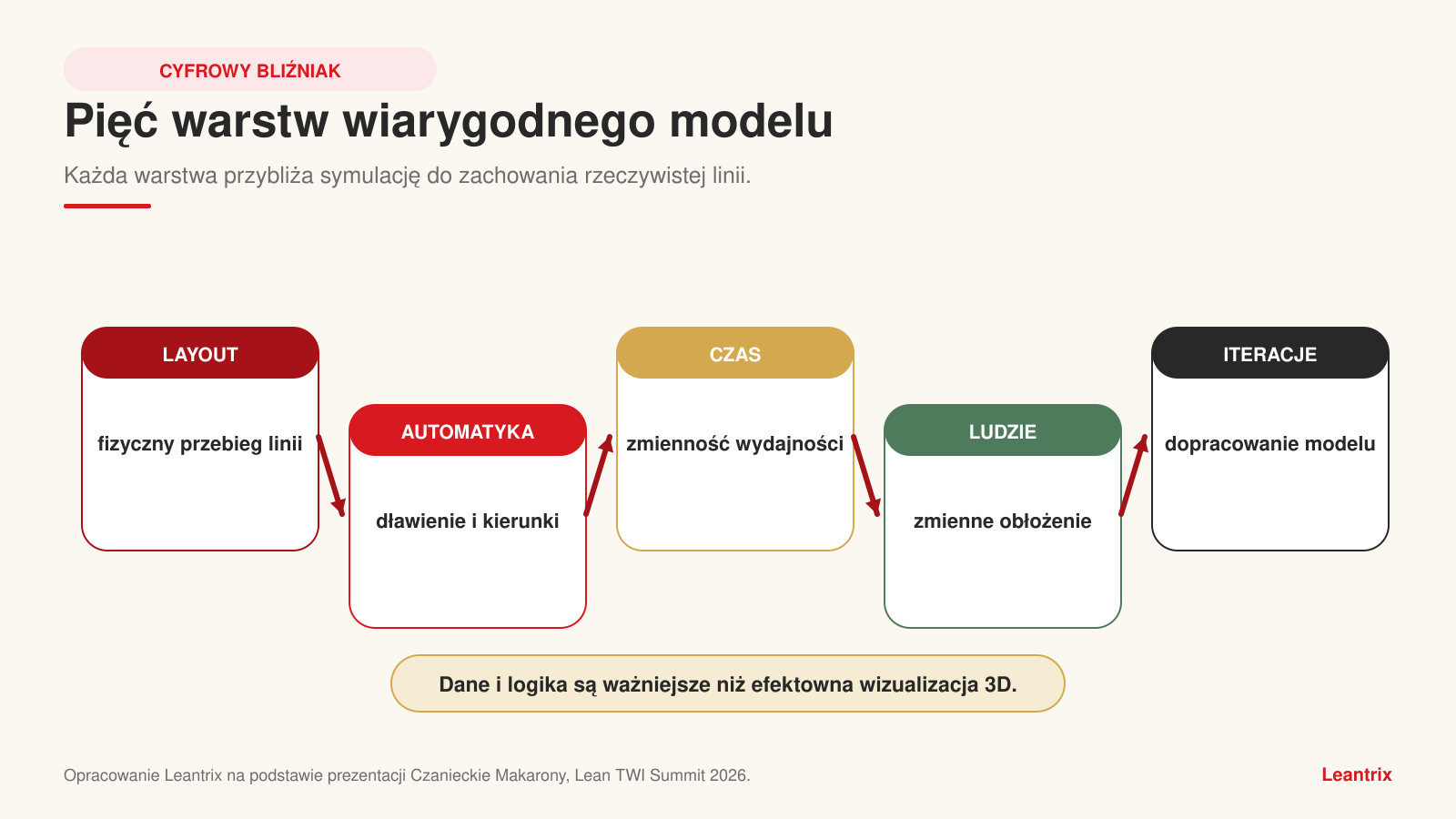
A digital twin is only as good as its assumptions and data. At Czanieckie Makarony, the model combined five layers: physical layout, automation logic, process behaviour over time, workforce availability and iterative refinement. Omitting any layer could produce an apparently precise but incorrect answer.
- Layout defined the sequence and connections between workstations.
- Automation logic reproduced actual control rules rather than nominal cycle times alone.
- Variability over time showed how deviations accumulated and travelled through the flow.
- Workstation staffing captured the effect of workforce availability on line behaviour.
- Model iterations progressively removed discrepancies between the simulation and MES data.
In practice, the most valuable project work is often invisible on the screen. It concerns event definitions, data quality, control rules and exceptions. A 3D model can make discussions easier, but process logic determines its credibility.
Validation revealed a change hidden in aggregate results
An unexpected effect emerged during validation. The model helped identify a process change that could not be clearly recognised from aggregated production results alone. The source anonymises the exact event date, so this article does not disclose it.
This is an important lesson for OEE analysis. The indicator shows that a result changed but does not always explain exactly what happened in the process sequence. Comparing the model with actual data can act as a consistency test: when simulation and reality diverge, investigate changes in standards, parameters, staffing or control logic.
Improving OEE: what the two scenarios showed
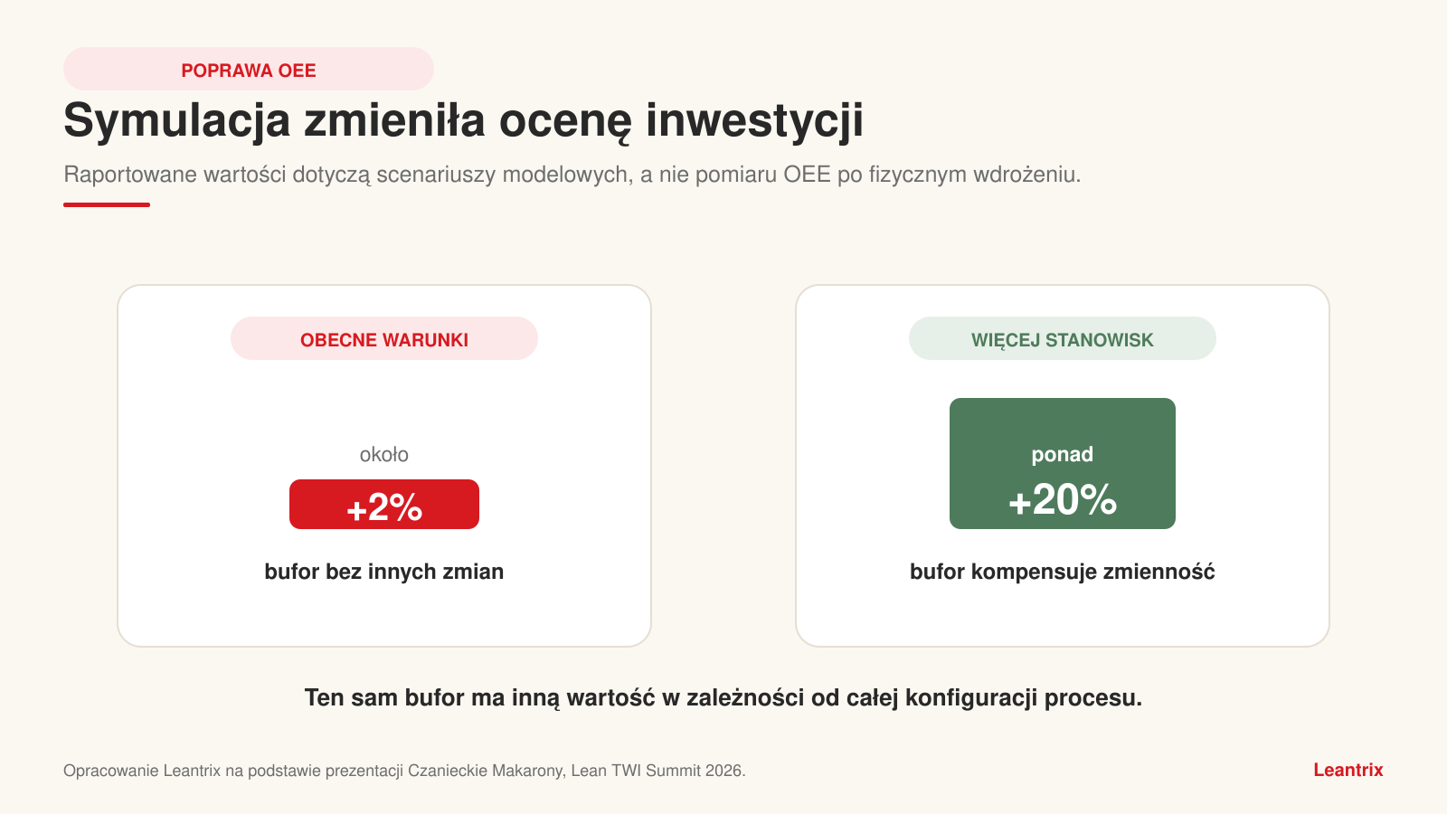
The simulation’s main result was a changed assessment of the investment. Under current production conditions, the buffer alone increased total throughput by approximately 2%. This was positive but far smaller than might be expected from an appraisal that ignored overall variability.
The buffer’s value became substantially greater only after the number of workstations was increased. In that scenario, total throughput rose by more than 20%, because the buffer could compensate for typical process variability. The solution was therefore neither inherently good nor bad; its effectiveness depended on the configuration of the entire system.
| Scenario | Reported simulation result | Decision implication |
|---|---|---|
| Buffer under current conditions | approximately 2% increase in total throughput | The buffer alone does not remove the main constraint |
| Buffer after increasing the number of workstations | more than 20% increase in total throughput | The buffer gains value when it can compensate for system variability |
What the simulation result establishes
Precise descriptions of evidence matter for a credible case study. The presentation confirmed 99% agreement between the model and actual data, alongside the results of two simulation scenarios. It did not present a final measurement following the physical implementation of all changes or before-and-after OEE values.
- Confirmed by the source: sources of variability, model construction, validation against MES data, 99% agreement and simulated results of approximately 2% and more than 20%.
- Decision implication: the investment scope should account for the relationship between the buffer and the number of workstations.
- Not established by the source: final OEE improvement after implementation, the period over which results were sustained, investment expenditure or payback time.
Here, improving OEE therefore provides an improvement direction and a decision criterion. To confirm the effect after investment, the company should remeasure availability, performance and quality, then compare the result with the baseline and model assumptions.
Improving OEE: six lessons for FMCG plants
The case can be translated into six practical principles relevant to other food-production plants.
- Define the decision first. A model should answer a specific business question rather than exist simply because the technology is available.
- Preserve variability instead of replacing it with one average. Keep event sequences, durations and workstation interdependencies.
- Validate against representative periods. A strong week and a weak week may reveal constraints hidden by an average day.
- Test combinations of changes. One element may have little effect alone but become valuable after another constraint changes.
- Separate model results from implementation outcomes. Simulation supports a decision; post-implementation measurement confirms whether the organisation achieved the expected effect.
- Treat discrepancies as information. A model losing its fit with reality may signal a process change worth investigating.
Managing a project from data to decisions
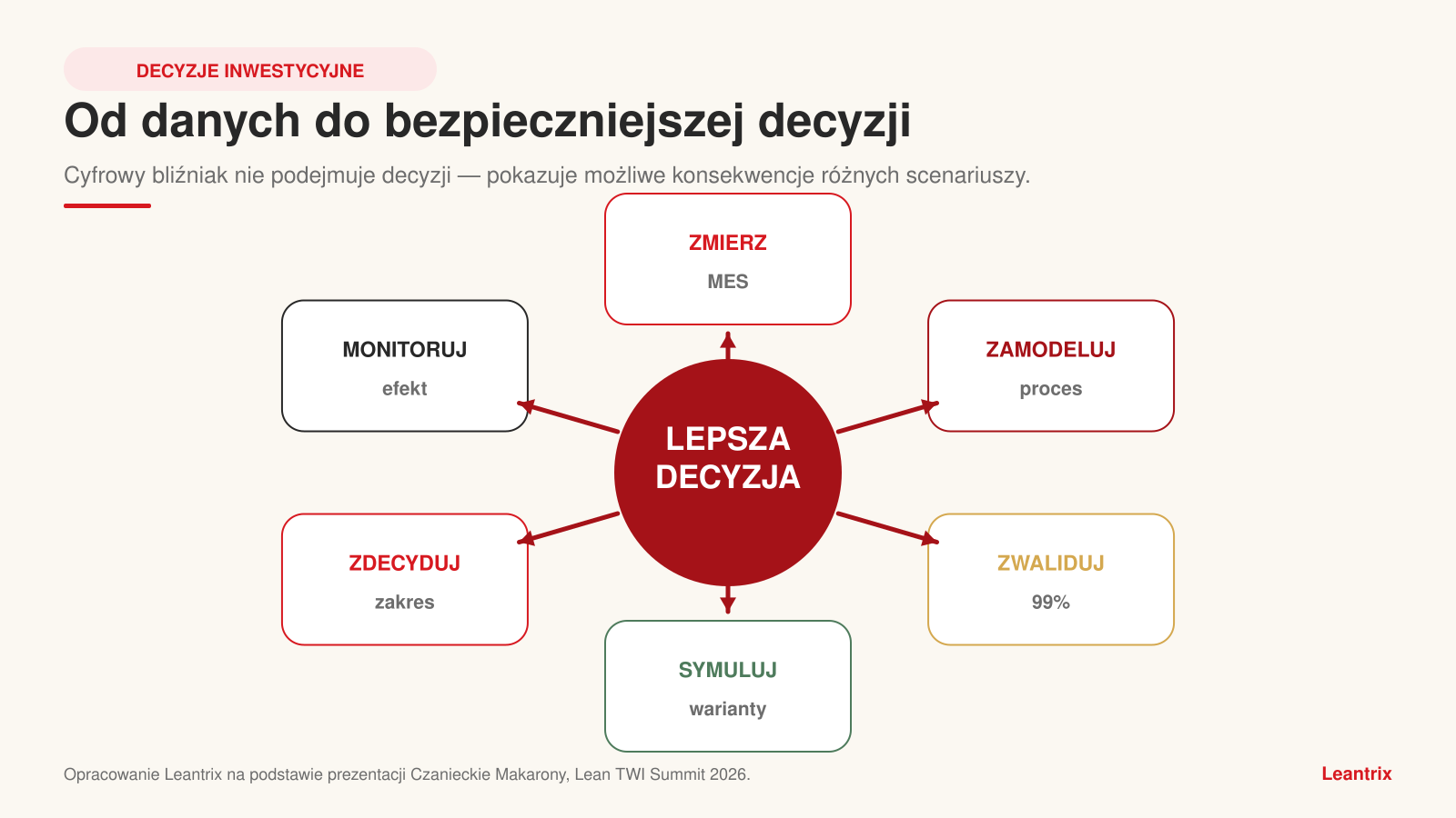
A practical path starts with selecting a problem and assigning an accountable decision owner. The team then defines process boundaries, data sources and the minimum accuracy needed for the intended use. Not every model needs the same detail; it must be good enough to distinguish the scenarios being analysed.
- Measure: establish event definitions and check MES data quality.
- Model: reproduce flow, control logic, staffing and variability.
- Validate: compare the model against several periods of actual operation.
- Simulate: test individual solutions and combinations.
- Decide: select the investment option, scope and boundary conditions.
- Monitor: compare actual results with forecasts after implementation and update the model.
Measuring the effect after implementation
To close the learning loop, the measurement plan should be prepared before introducing the change. Otherwise, an organisation may achieve greater volume without knowing whether it came from the investment, a different product mix, increased staffing or an unusually stable period.
| Area | Example measure | Purpose |
|---|---|---|
| Availability | planned time, breakdowns and minor stoppages | check whether the investment reduces lost operating time |
| Performance | actual pace against the standard | assess the effects of throttling and workstation variability |
| Quality | right-first-time production | ensure higher speed does not impair quality |
| Flow | total throughput, WIP and buffer occupancy | observe the entire line rather than only local machines |
| Economics | investment cost, savings and payback | confirm the business decision’s value |
The best measurement plan compares periods with similar product mix, staffing and demand. It should also allow time for the new working method to stabilise. One good week is a signal rather than evidence of a lasting effect.
Common mistakes in using a digital twin
- Modelling an ideal process. Excluding breakdowns, breaks, staffing changes and exceptions exaggerates the predicted effect.
- Validating against a single day. An unusually stable period can hide differences present in normal work.
- An excessively detailed initial model. The team spends too long reproducing elements that do not affect the decision.
- No data owner. Different definitions of downtime or good product prevent reliable comparison.
- Testing only one option. The largest effect may require combining several changes.
- No post-implementation measurement. The organisation cannot tell whether reality confirmed the model or what to learn for the future.
Lessons from Czanieckie Makarony’s case study
The central lesson is the relationship between a solution and its system. A buffer can deliver approximately 2% or more than 20% greater total throughput, depending on the other constraints remaining in the process. This difference is too large to base a decision solely on a static spreadsheet and nominal cycle times.
Improving OEE therefore begins with a reliable picture of work. MES data shows events, the model structures relationships, validation builds confidence and simulation enables safe scenario comparison. Technology supports managerial accountability by providing better evidence for decisions.
FAQ: improving OEE and digital twins
Does a digital twin automatically improve OEE?
No. A model does not change the physical process. It helps identify the right course of action, estimate its impact and reduce investment risk. The effect must then be achieved through implementation and confirmed by actual measurement.
Why is average line productivity insufficient?
An average removes the sequence of events. It does not show whether short stoppages coincide, how staffing changes or when one workstation throttles another. In a connected process, these relationships often determine total capacity.
What does 99% model agreement mean?
It is the level of fit between simulation and actual MES data reported in the presentation. It does not mean every future forecast will be exactly 99% accurate. The model must be updated when the process, product mix, staffing or control rules change.
Was the increase of more than 20% achieved after implementation?
The presentation describes a modelled scenario involving a buffer after increasing the number of workstations. It does not present a final post-implementation OEE study. The figure should therefore be read as the result of a credible simulation supporting a decision, rather than a claimed outcome of physical implementation.
About the case study presenter
Patryk Dybał is an authorised commercial representative and General Manager at Czanieckie Makarony. At Lean TWI Summit 2026, he presented a practical application of a digital twin to evaluate an investment intended to increase production-line capacity. He showed how combining process knowledge, MES data and simulation can reduce decision risk and reveal relationships hidden in aggregated production results.
This article is based on materials presented by Czanieckie Makarony at Lean TWI Summit 2026 in Wrocław. The graphics are original, simplified illustrations by Leantrix; they do not reproduce the plant’s detailed layout or confidential process parameters.